What is IFERROR in Google Sheets?

IFERROR allows you to handle errors that occur while performing calculations or formulas. It provides a way to replace these errors with specified values or even perform alternative calculations when an error is encountered. This ensures that your spreadsheet remains error-free and your data remains accurate.

The IFERROR function checks if an error occurs in a formula or calculation and provides an alternative value if true. It can handle various types of errors such as #DIV/0!, #VALUE!, #REF!, #NAME?, #NUM!, and #N/A. By using this function, you can prevent error messages from cluttering your sheet and display meaningful values instead.

Simply put, IFERROR helps you turn this:

into this:

How to use the IFERROR function in Google Sheets

The syntax of the IFERROR function is very simple:

=IFERROR(value, value_if_error)

It only takes two parameters: value and value_if_error

• value: This is the value or formula that you want to evaluate for any errors.
• value_if_error: Optional. This is the value you want to display if there is an error in value.

So, for example, the following formula will try to calculate 1/0 (which will lead to a division-by-0 error) and instead display "I'm afraid I can't do this."

=IFERROR(1/0, "I'm afraid I can't do this.")

"If no error"

The second parameter is optional, so if you just want to handle the error without displaying any specific message or value, you can omit the second parameter in the IFERROR function. This way, the function will simply return a blank cell when an error occurs. For example:

=IFERROR(1/0)

Now the IFERROR function will return a blank cell instead of displaying an error message. This can be useful when you don't need to explicitly notify the user of the error, but rather want to handle it silently. But reading the function now becomes a bit confusing. As now the function will actually output results if there is no error.

Examples

Let's look at three more complex, real-life examples.

Get rid of #DIV/0! errors

Let's say you have a worksheet that calculates the average revenue per customer. However, sometimes there may be zero customers, resulting in a division by zero error.

To handle this situation gracefully, you can use the IFERROR function.

=IFERROR(C2/B2, 0)

In this example, B contains the number of months somebody has been a customer, and C contains the cummrevenue from that customer. The IFERROR function calculates the average revenue per month for each customer by dividing the total revenue by the number of months.

If there is a division by zero error, the IFERROR function replaces it with a zero. This ensures that your sum and average revenue per customer calculation doesn't break due to new customers who have 0 months of revenue recorded.

Catch errors in ARRAYFORMULA()

Let's simplify our table. Did you know you can use ARRAYFORMULA to fill a hole column with the results from a calculation?

Simply enter into E2 the following formula:

=ARRAYFORMULA(C2:C10/B2:B10)

This will fill the remaining cells with the results from that calculation.

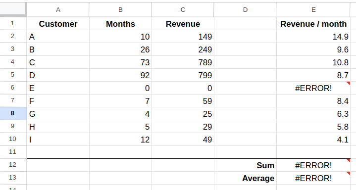
But of course, the #DIV/0! error has returned. You might have guessed it, by wrapping our division in the IFERROR function, we can catch those errors and simply ignore that row in our calculations.

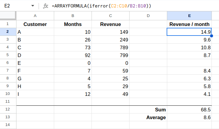
But now the average has changed. What has happened? Because we didn't define a default value in the IFERROR function, it now simply returns an empty cell. The AVERAGE function ignores empty cells.

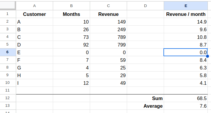
If we want to have the IFERROR function output 0 as before, we need to define 0 as the default value if there is an error.

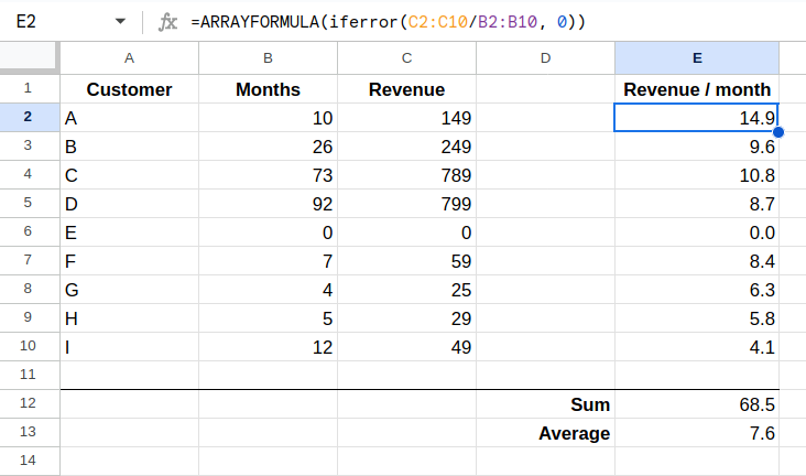
Now the average calculation will incorporate the 0 and produce a lower average.

Handle errors in lookup functions:

Lookup functions like VLOOKUP or INDEX/MATCH return errors when the specified lookup value is not found. You can use the IFERROR function to display a custom message or value instead of an error message. For instance:

=IFERROR(VLOOKUP(A1, C1:H25, 2, FALSE), "Value not found")

In this example, the VLOOKUP function looks for the value in cell A1 within the specified range. If the value is not found, the IFERROR function will display "Value not found" instead of an error.

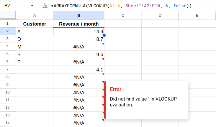
If we add a new sheet with a VLOOKUP function to our example from above, and use an ARRAYFORMULA, it would quickly produce lots of errors:

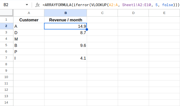
But again, if we surround the VLOOKUP with IFERROR and simply don't specify a default value, we get empty rows for customers that aren't in our list or for empty fields.

These are just a few examples of how the IFERROR function can be used to handle errors in Google Sheets. By incorporating IFERROR into your formulas, you can ensure that your spreadsheet calculations are more robust and user-friendly, providing accurate results even in the presence of potential errors or missing data.

Types of errors

The IFERROR function in Google Sheets can catch various types of errors that commonly occur in spreadsheet calculations. Here are some of the types of errors that IFERROR can handle:

#DIV/0! error

This error occurs when you divide a number by zero, which is mathematically undefined.

#N/A error

This error is often encountered when using lookup functions like VLOOKUP or INDEX/MATCH. It signifies that the specified lookup value is not found in the lookup range.

#VALUE! error

This error occurs when there is an issue with the input values or the data type is not compatible with the formula.

#REF! error

This error arises when a formula refers to a cell or range that has been deleted or removed.

#NAME? error

This error typically occurs when a formula contains a misspelled function name or refers to a function that does not exist.

#NUM! error

This error is encountered when a formula encounters an invalid numeric value or an unexpected character.

#NULL! error

This error occurs when a range intersection is attempted but no overlapping range is found.

Alternatives

While the IFERROR function is a powerful tool for error handling in Google Sheets, there are alternatives available for handling errors in spreadsheet calculations. Here are a few alternatives you can consider:

The good old IF statement

The IF statement allows you to perform different actions based on a specified condition. Instead of using IFERROR to handle errors, you can use an IF statement to check for errors explicitly and provide customized responses or alternative calculations based on the condition. However, this approach can make your formulas more complex and lengthy compared to using IFERROR.

Conditional formatting

Conditional formatting is a feature in Google Sheets that allows you to format cells based on specific rules or conditions. While it doesn't directly handle errors, you can use conditional formatting to highlight or visually identify cells with errors. This can help you quickly identify and rectify the errors manually. However, it doesn't provide an automated way to replace error values with custom messages or alternative calculations.

ISERROR or ISERR

The ISERROR and ISERR functions can be used to check whether a cell or formula returns an error. These functions return either TRUE or FALSE based on whether an error is present. You can combine these functions with IF statements to handle errors and provide custom responses. However, this approach requires more complex formulas and manual customization for each error type.

ISNA

Another alternative way to handle errors in Google Sheets is to use the ISNA function. ISNA stands for "is not available" and is specifically designed to check if a cell or formula returns the #N/A error.

Here's how you can use the ISNA function as an alternative to IFERROR:

1. Use ISNA within an IF statement: =IF(ISNA(A1), "Custom message or value", A1) This formula checks if cell A1 returns the #N/A error. If it does, it displays a custom message or value. Otherwise, it simply returns the value in cell A1. You can replace "Custom message or value" with any message or value of your choice.

2. Combine ISNA with other error-checking functions: You can combine ISNA with other functions like IF, VLOOKUP, or INDEX/MATCH to specifically handle the #N/A error in those formulas. Here's an example using the VLOOKUP function: =IF(ISNA(VLOOKUP(A1, C1:H25, 2, FALSE)), "Value not found", VLOOKUP(A1, C1:H25, 2, FALSE)) In this formula, ISNA checks if the VLOOKUP function returns the #N/A error. If it does, it displays "Value not found". Otherwise, it returns the result of the VLOOKUP function.

The ISNA function is particularly useful when you want to focus on the #N/A error and handle it differently from other error types. It gives you more control over how you want to handle the #N/A error specifically, while other error-handling techniques like IFERROR handle all error types uniformly.

Consider your specific error-handling needs and choose the technique that best suits the nature of the errors you encounter in your spreadsheet calculations.